Integration by Parts

Ok here it is! This is what we've all been waiting so long for! The blog post for how to do integration by parts! I know its a bit late but only by 3 weeks.

Integration by parts was basically created with the idea of the product rule in mind. If you have two things being multiplied, you can take the derivative of each separate piece and it would be the same as taking the derivative of the whole thing. Guess what! It works the same way with integrals too! Fancy that, its funny how the world works.

So basically we start out with the equation:

And by the magic of math it is simplified to:

So lets say your trying to integrate

xcosxdx

The first thing you would do is pick a u and a dv.
u=x dv=cosxdx
Which means that
du=dx v=sinx

Then plug it into the equation so you will have

This you can then easily simplify to xsinx-cosx+C

The thing to remember is not every u and v combination will work so if it appears that one just makes the new equation more complicated, stop and start over with a different set of u's and v's. Try and make u something that simplifies when its differentiated, and try to make dv something that remains manageable when its integrated. One easy way to remember what to look for in integrals is by using the phrase:

L n

I nverse Trig

P olynomials

E xponentials

T rig

Sometimes during your mathematical travels you will come across some integrals in which you would have to use integration by parts twice. Basically all you do is do integration by parts once, and then do integration by parts again, but only for the part of the answer that still has to be integrated. Then you can just put that answer back in.

Lastly, we learned one more form of integration. Its called Tabular Integration and its basically the cheating way of integration by parts. In your integral, if you have one piece that if differentiated enough times will end up at 0, and the other piece is easy to integrate over and over and over, then you can just put them in tabular integration. Lets say you have the integral

So obviously the x squared part is the part that is easy to differentaite and the e to the x is the part that can be integrated many times over. So you make a list where in the write column you begin with the x squared and differentiate it until it is zero. Then on the other side integrate the e to the x until you have it lined up with the zero. Then do a diagonal line from the first x squared to the integral of e to the x and keep making those lines until you run out of e to the x's. Then make the first one positive, the second one negative, the third one positive, and so on. That there is a mediocre account of tabular integration since I was unable to use any diagrams, so if you have questions (which I doubt) ask me in person and I will show you.

Logistic Growth and Partial Fractions 1/22/08

Hi!
We have a test on integration Fri. 1/25 (which is also a food day!)
To review - pg. 358 #'s 1-28
Partial Fractions HW due Tues - pg.452 #'s 7-29 odd

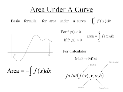
Area Under A Curve

Sorry this is late, but we had this lesson on Wed, Nov 27, 2007

For some practice problems, go to page 264 and do Exploration 1
Homework: pg 254 #5-13 odd, 20; pg 267 #7-41 odd

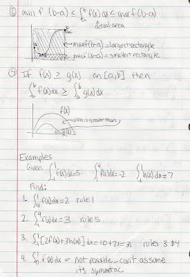
Integrals

Hi Everyone!
This Friday (11/30) is food day! Please bring whatever you decided you were going to because otherwise we'll all be sad (and hungry).
Homework: pg. 274 #'s 1-33 odd
We took lots of notes today - here are scanned copies (to enlarge click on them).

Newton's Method , Differentials, Related Rates

Hi guys
we have Quiz on Nov 6th, Tuesday.

Newton's Method
The general method

More generally, we can try to generate approximate solutions to the equation using the same idea. Suppose that is some point which we suspect is near a solution. We can form the linear approximation at and solve the linear equation instead.
That is, we will call the solution to . In other words,

If our first guess was a good one, the approximate solution should be an even better approximation to the solution of . Once we have , we can repeat the process to obtain , the solution to the linear equation

Solving in the same way, we see that

Maybe now you see that we can repeat this process indefinitely: from , we generate and so on. If, after n steps, we have an approximate solution , then the next step is

Provided we have started with a good value for , this will produce approximate solutions to any degree of accuracy.


Dfferentials

Given a function we call dy and dx differentials and the relationship between them is given by

Note that if we are just given then the differentials are the df and dx and we compute them the same manner

Related Rates

There is 13ft of string beteen two people. The people holding the string.

One person(x) is moving left and another person (Y)is moving forward. (keeping the distance between people 13ft)

speed of Y person is 4ft/s

We can know that the length of x side is 5ft and length of y side is 12ft to use pythagorean theaorem.

2 2 2

x + y = 13

2x (dx/dt) + 2y (dy/dt) = 0

x(dx/dt) + y(dy/dt) = 0

x(dx/dt) + y*4 = 0

5(dx/dt) + 12*4 = 0

dx/dt = - 9.6

Mean Value Theorem Applications, First Derivative Test

So this is Jake. Basically, Mr. Marchetti extrapolated on the Mean Value Theorem (grrr theorem). Anyways, the homework he gave us was page 192 # 1-13 odd, 19-37 odd, 42, and 43. Also, he postponed the quiz until Tuesday the 23rd, so cram for that while you're at it.

Now, the MVT (Mean Value Theorem) has 3 basic premises that apply.
1. The Increasing/Decreasing Rule
So this rule basically states that, and I quote, "If, over the course of the interval, the secant line's slope is positive, then the tangent line's slope will also be positive."
In literal terms, this means that when the function is increasing, the secant line, and therefore the tangent line's slopes will be positive.



What this means to us is that functions increase when f'(x) > 0 and they decrease when f'(x) <0

The second rule is that a line with a derivative of zero is constant, so x=5 is just a horizontal line.

The third rule of the MVT is that "3. Functions with the same derivative only differ by a constant." Therefore, if f'(x) = g'(x), then f(x) = g(x) + constant
Here is an example for you: we have both f'(x) and g'(x) equaling 2x
You know that f(x) must = x^2 and that g(x) must also = x^2. However, g(x) could also equal x^2 + 121. That would still result in a derivative of 2x, the same as for f'(x), proving that functions with identical derivatives only differ by a constant.

Now that we have the MVT explained, we can move onto the First Derivative Test. What this rule states is that "When the derivative goes from positive to negative, you have a max. When the derivative goes from negative to positive, you have a min. And finally, if the derivative doesn't change signs, then there is no max or min." Pretty self-explanatory.

In this graph right here, you can see that, at -2, the derivative is negative and then switches to positive. This shows that there is a relative minimum at that point. At -1, the derivative is positive and goes to negative, leading there to be a maximum at that point.

To put all of this together, there is a good example that Mr. Marchetti showed to us on the board. You have the function y= x^3 - 4x. You need to find the maximum(s) and minimum(s). Ready go. So to solve this, you need to first find the equation's derivative. That is y' = 3x^2 - 4. You make that equation equal to 0 in order to determine where the critical points are in this specific function.
0 = 3x^ - 4
4 = 3x^2
4/3 = x^2
+/- (4/3)^.5 = x (this would be a lot less cluttered if I could insert stuff...)
+/- 2 / (3)^.5 = x

Now that you have the critical points of the function (where the derivative changes signs, which results in a max or a min as stated in the First Derivative Test), you can figure out how the function's derivative behaves in each interval. The intervals that you will have in this instance will be (- infinity, -2/(3)^.5), (-2/(3)^.5, 2/(3)^.5), and (2/(3)^.5, infinity). What you do is pick any value within each interval and plug that into the derivative equation that you found earlier (3x^2 - 4) to find how the derivative in that interval behaves. Remember, the endpoints of each interval are 0's, so the derivative crosses the x axis at those points and changes signs.
(- infinity, -2/(3)^.5)...: 3(-5)^2 - 4 = 71, positive in this interval
(-2/(3)^.5, 2/(3)^.5)...: 3(0)^2 - 4 = -4, negative in this interval
(2/(3)^.5, infinity)...: 3(5)^2 - 4 = 71, positive in this interval
now, to find which of these critical points is the maximum and which is the minimum, you refer again to the First Derivative Test. It states that when the derivative goes from positive to negative, you have a maximum. Therefore, at the point -2/(3)^.5), you have a maximum. Also, because the First Derivative Test states that when the derivative goes from negative to positive, you have a minimum, you know that your minimum is at 2/(3)^.5.

That is all that was talked about in class on Wednesday. Again, we'll see if the inserting pictures problem resolves itself or not.

SCRIBE POST - OCTOBER 10, 2007

Hi guys, it's Devon. I was the scribe last Wednesday (October 10). It was a late start day, so all we covered was something called The Mean Value Theorem. We recieved a review packet, and we had to start working on that in preperation for our quiz Friday, October 19th.

Ok. Here we go.

The Mean Value Theorem connects the average rate of change and instantaneous rate of change of a function. The theorem states that all continuous and differentiable points between A and B on a differentiable curve, have at least one tangent line parallel to AB.



Between points A and B, we find a point C. Point C is the point of a parallel tangent line, and can be found by the previous equation.

A graph that represents The Mean Value Theorum would look like this:



An example of this would be driving. If you went on a 3 hour trip, averaging about 30 miles/hour, The Mean Value Theorem states that you would have to be going exactly that speed at least one time in the duration of your drive. That's basically it, it's pretty simple.